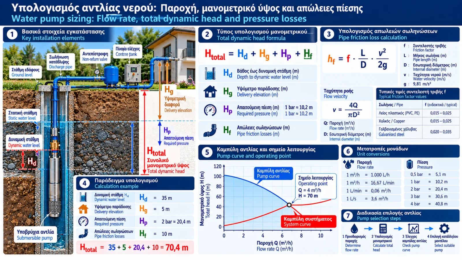
Water Pump Sizing: Flow Rate, Total Dynamic Head and Pressure Losses

Correct water pump selection cannot be based solely on motor power or the maximum pressure listed in a product catalogue.

For a water system to operate reliably, the pump must deliver the required quantity of water at the pressure needed by the installation.

This requires calculating two fundamental parameters: flow rate Q and total dynamic head H.

Pressure losses through pipes, valves, filters and other fittings must also be considered.

This Thermosphere.gr technical guide explains the sizing process with equations, conversion tables and worked examples.

1. What Does Water Pump Sizing Mean?

Pump sizing is the process of determining the hydraulic requirements of an installation and selecting equipment capable of meeting them.

The main inputs include:

• Required water flow.

• Elevation differences.

• Required delivery pressure.

• Pipe length and diameter.

• Fittings and valves.

• Water source characteristics.

• Pump performance curves.

The objective is to select a pump that operates within an appropriate region of its performance curve, avoiding unnecessary energy consumption and mechanical stress.

2. What Is Pump Flow Rate?

Flow rate is the volume of water delivered per unit of time.

It is represented by Q.

Common units include:

• m³/h.

• L/min.

• L/s.

Useful conversions:

1 m³/h = 1,000 L/h = 16.67 L/min

1 L/s = 3.6 m³/h

Example

A water installation requires 50 litres per minute.

Q = 50 × 60 / 1,000

Q = 3 m³/h

The pump must therefore be capable of delivering 3 m³/h at the required head.

3. How Is Required Flow Determined?

The method depends on the application.

In buildings, required flow depends on fixture demand and the probability of simultaneous use.

Adding the maximum flow of every fixture is not always appropriate because all fixtures may not operate simultaneously.

Suitable peak-demand calculation methods should be used according to applicable standards and local requirements.

For irrigation, flow is often determined by the total demand of the active irrigation zone.

For example, 20 drippers rated at 4 L/h require:

Q = 20 × 4 = 80 L/h

Therefore:

Q = 0.08 m³/h

The operating pressure required by the irrigation equipment must also be considered.

4. What Is Pump Head?

Pump head represents the hydraulic energy added to water per unit weight.

It is represented by H and expressed in metres.

In a simplified installation, required head can be calculated as:

H = Hgeo + Hp + Hloss

Where:

• Hgeo = static elevation difference.

• Hp = required pressure head.

• Hloss = total hydraulic losses.

This simplified relationship assumes appropriately selected reference points and negligible velocity-head differences or that those terms are already included.

A more general analysis uses the complete energy equation.

5. Converting Pressure from Bar to Metres of Water

For water with a density of approximately 1,000 kg/m³ and gravitational acceleration of 9.81 m/s²:

1 bar ≈ 10.2 metres of water column

Similarly:

10 metres of water ≈ 0.981 bar

Conversion Table

Values are approximate and depend on liquid density.

6. What Is Static Elevation Head?

Static elevation head is the vertical difference between the appropriate source and delivery reference points.

For a simple transfer between two open tanks, it is the difference between their free water surfaces.

For example, if the source tank surface is at elevation 0 m and the destination tank surface is at 15 m:

Hgeo = 15 m

In borehole applications, the appropriate dynamic water level is used for the required pumping rate.

Total borehole depth is not automatically equal to static pumping head.

7. What Are Pipe Friction Losses?

As water moves through pipes, energy is lost due to friction.

These losses depend on:

• Pipe length.

• Internal diameter.

• Flow rate.

• Water velocity.

• Pipe roughness.

• Water viscosity.

As flow increases through a given pipe, friction losses generally increase substantially.

Selecting an undersized pipe can increase required pump head and energy consumption.

8. The Darcy–Weisbach Equation

A fundamental equation for pipe friction head loss is:

hf = f × (L/D) × (v²/2g)

Where:

• hf = friction head loss, m.

• f = Darcy friction factor.

• L = pipe length, m.

• D = internal pipe diameter, m.

• v = mean flow velocity, m/s.

• g = gravitational acceleration, approximately 9.81 m/s².

The friction factor depends on Reynolds number and relative pipe roughness.

For laminar flow in a circular pipe, f = 64/Re.

For turbulent flow, suitable correlations or diagrams can be used, including Colebrook–White and its approximations.

9. How Is Water Velocity Calculated?

Mean water velocity is:

v = Q/A

For a circular pipe:

A = πD²/4

Therefore:

v = 4Q/(πD²)

When using SI units, flow must be in m³/s and diameter in metres.

Example

Assume:

• Q = 3 m³/h = 0.000833 m³/s.

• Internal diameter D = 0.032 m.

Then:

A ≈ 0.000804 m²

and:

v ≈ 1.04 m/s

This velocity can then be used to estimate pipe friction losses.

10. Example: Calculating Pipe Friction Losses

Assume:

• Flow rate: 3 m³/h.

• Pipe length: 50 m.

• Internal diameter: 32 mm.

• Water velocity: approximately 1.04 m/s.

• Assumed Darcy friction factor: f = 0.025.

Then:

hf = 0.025 × (50/0.032) × (1.04²/(2 × 9.81))

hf ≈ 2.15 m

In this hypothetical example, straight-pipe friction losses are approximately 2.2 metres of water head.

For an actual installation, the friction factor must be determined from flow and pipe characteristics.

Local fitting losses are not yet included.

11. What Are Minor or Local Losses?

In addition to straight-pipe friction, losses occur through:

• Elbows.

• Tees.

• Valves.

• Non-return valves.

• Contractions and expansions.

• Inlets and outlets.

• Filters.

For many fittings, local head loss can be estimated by:

hm = K × v²/(2g)

Where K is the local resistance coefficient.

K depends on fitting geometry and operating conditions.

For filters and specialised components, manufacturer pressure-drop curves are often preferable.

12. Complete Example: Sizing a Domestic Water Pump

Consider a hypothetical installation with:

• Required flow: 3 m³/h.

• Elevation difference from source water level to delivery point: 12 m.

• Required delivery pressure: 2 bar.

• Straight-pipe friction losses: 4 m.

• Local fitting losses: 3 m.

The required pressure head is:

Hp ≈ 20.4 m

Total head:

H = 12 + 20.4 + 4 + 3

H = 39.4 m

We therefore need a pump capable of delivering:

Q = 3 m³/h at H ≈ 39.4 m

This must be verified using the manufacturer's pump curve.

A pump with a maximum head of 40 m is not automatically suitable, because that maximum may occur at nearly zero flow.

13. How to Read a Pump Performance Curve

The Q–H curve shows the relationship between flow rate and pump head.

Flow Q is generally shown on the horizontal axis.

Head H is shown on the vertical axis.

For many centrifugal pumps, available head decreases as flow increases.

Manufacturers may also provide:

• Efficiency curves.

• Absorbed power curves.

• Required NPSH curves.

• Permitted operating ranges.

All relevant performance information should be considered during selection.

14. What Is the Operating Point?

The operating point is determined by the intersection of the pump curve and system curve.

The system curve represents the head required at different flow rates.

For a simplified system with constant static head:

Hsystem(Q) = Hstatic + Hloss(Q)

Hydraulic losses increase with flow.

The actual operating point is not determined by the pump alone or by the pipework alone.

It results from their interaction.

15. What Is the Best Efficiency Point?

BEP stands for Best Efficiency Point.

It is the operating point at which the pump reaches its maximum hydraulic efficiency under specified conditions.

Operating near BEP is often desirable because it may provide:

• Lower energy consumption.

• Reduced hydraulic stress.

• Better operating behaviour.

• Improved reliability.

However, not every installation must operate exactly at BEP.

The manufacturer's preferred and allowable operating ranges should be followed.

16. How Is Hydraulic Power Calculated?

Hydraulic power is calculated using:

Ph = ρ × g × Q × H

Where:

• Ph = hydraulic power, W.

• ρ = water density, approximately 1,000 kg/m³.

• g = 9.81 m/s².

• Q = flow rate, m³/s.

• H = head, m.

Example

For:

Q = 3 m³/h = 0.000833 m³/s

H = 40 m

Ph = 1,000 × 9.81 × 0.000833 × 40

Ph ≈ 327 W

This is the hydraulic power delivered to the water, not the electrical input power.

17. How Is Electrical Input Power Estimated?

Electrical input power depends on overall system efficiency.

For a simplified calculation:

Pe = Ph / ηtotal

Assume an overall efficiency of 50%:

Pe = 327 / 0.50

Pe ≈ 654 W

This is an illustrative value.

Actual efficiency depends on the pump, motor and any electronic drive.

Motor rated power should not simply be equated with calculated electrical input.

Required shaft power, motor characteristics and operating limits must also be assessed.

18. Example: Sizing a Borehole Pump

Assume:

• Dynamic water level: 35 m below ground.

• Delivery point: 5 m above ground.

• Required delivery pressure: 2 bar.

• Pipe friction and fitting losses: 10 m.

• Required flow: 4 m³/h.

Elevation difference:

35 + 5 = 40 m

Required pressure head:

2 bar ≈ 20.4 m

Total head:

H = 40 + 20.4 + 10

H ≈ 70.4 m

The pump must therefore deliver:

Q = 4 m³/h at H ≈ 70.4 m

The borehole must also be capable of sustaining this flow without excessive drawdown.

19. Common Water Pump Sizing Mistakes

Selecting Only by Horsepower

Motor power alone does not define flow and head.

Using Maximum Catalogue Flow

Maximum flow often occurs at very low head.

Using Maximum Catalogue Head

Maximum head often occurs near zero flow.

Ignoring Pipe Losses

Small pipe diameters and long distances can substantially increase required head.

Confusing Borehole Depth with Pump Head

Total borehole depth is not automatically the pumping head.

Ignoring Delivery Pressure

Water must reach the delivery point at sufficient pressure.

Ignoring Variable Operating Conditions

Demand, water level and system resistance can change.

20. Frequently Asked Questions

How Many Bar Is 30 Metres of Water Head?

Approximately 2.94 bar for water with a density close to 1,000 kg/m³.

How Many Metres of Head Is 4 Bar?

Approximately 40.8 metres of water column.

Can I Select a Pump Using Horsepower Alone?

No. Required flow and head must be checked against the pump performance curve.

Why Doesn't a 5-Bar Pump Deliver 5 Bar When a Tap Is Open?

Because maximum pressure may occur at zero or very low flow, while actual operation depends on demand and hydraulic losses.

How Do I Size a Pump for an 80-Metre Borehole?

You need dynamic water level, required flow, delivery elevation, required pressure and pipe losses.

Is a Bigger Pump Always Better?

No. An oversized pump may operate outside its preferred range, consume unnecessary energy and cause pressure or control problems.

How Can I Determine Actual Pump Flow?

By measuring flow with suitable equipment and comparing pressure conditions with the manufacturer's performance curve.

Conclusion

Correct water pump sizing requires a combination of hydraulic calculations.

Required flow is determined by demand, while total dynamic head depends on elevation difference, delivery pressure and hydraulic losses.

The pump performance curve confirms whether the required operating point is achievable and appropriate.

The right pump delivers the required flow at the required head with acceptable efficiency and reliable operation.

Technical References and Further Reading

• Hydraulic Institute: Pump system design and selection — https://www.pumps.org/

• Europump: Pump technology and efficiency resources — https://www.europump.net/

• KSB: Pump technical reference and performance curves — https://www.ksb.com/

• Grundfos: Pump sizing and technical education — https://www.grundfos.com/

• Darcy–Weisbach equation: Fundamental relationship for pipe friction losses.

• Colebrook–White equation: Relationship for estimating turbulent-flow friction factors.

• EN 806: Specifications for installations inside buildings conveying water for human consumption.

All numerical examples are hypothetical and should not be treated as ready-made installation specifications.

Note: Final sizing must be verified using actual installation data, manufacturer performance curves and applicable design requirements.

Thermosphere.gr — Technical knowledge for water supply and building systems.