
# Reverse Osmosis (RO) System Design: Flow, Pressure, Recovery and Calculations
## Introduction
The design of an industrial reverse osmosis (RO) system determines permeate quality, production capacity, membrane life, energy consumption and operating costs.
A reliable RO design requires more than selecting a nominal water production rate. Feedwater chemistry, temperature, osmotic pressure, scaling potential, hydraulic configuration and membrane operating limits must all be considered.
The calculations below are educational examples. Final engineering design requires a complete water analysis, membrane projection software and verification against manufacturer specifications.
## 1. Determining Required Permeate Production
The first step is to determine the required permeate production rate.
Design capacity should account for daily demand, available operating hours, redundancy and water losses associated with flushing or cleaning.
Example:
Daily permeate requirement: 120 m³/day.
Available production time: 20 hours/day.
Required production rate:
Qp = 120 / 20 = 6 m³/h.
Additional operating losses or availability limitations should be evaluated separately.
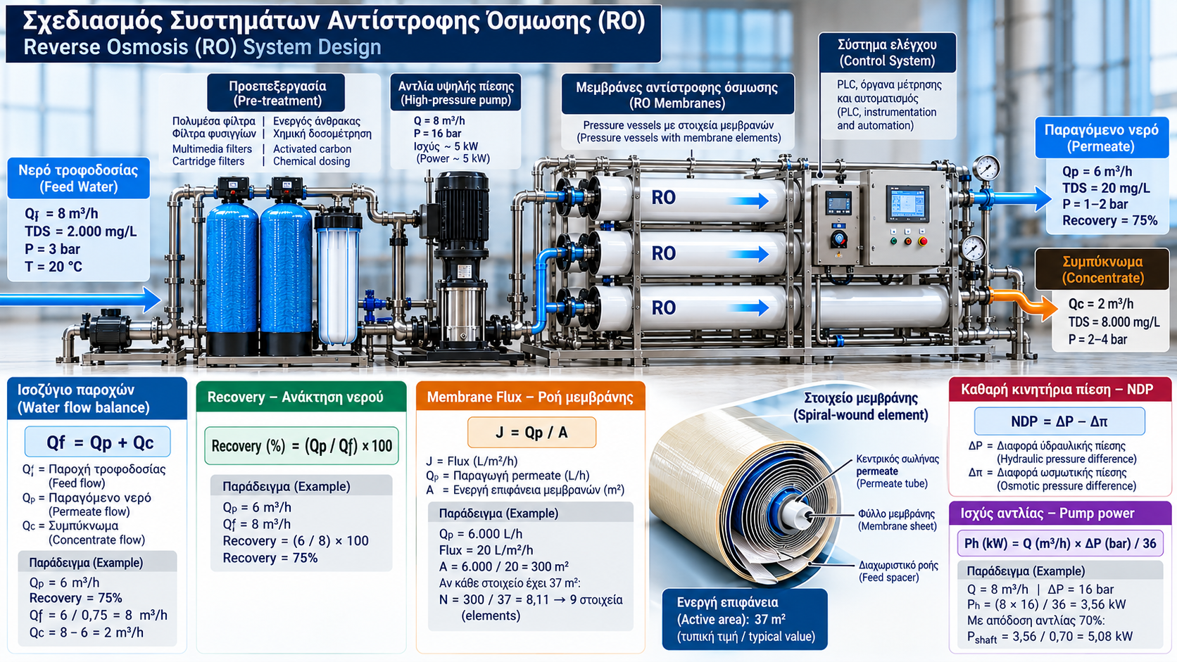
## 2. Water Flow Balance
An RO system separates incoming feedwater into permeate and concentrate.
Qf = Qp + Qc
Where:
Qf = Feedwater flow.
Qp = Permeate flow.
Qc = Concentrate flow.
This balance applies under steady-state conditions without additional flows crossing the selected system boundary.
## 3. Water Recovery
Recovery represents the percentage of feedwater converted into permeate.
Recovery (%) = (Qp / Qf) × 100
Example:
Permeate production = 6 m³/h.
Assumed recovery = 75%.
Qf = 6 / 0.75 = 8 m³/h.
Qc = 8 − 6 = 2 m³/h.
Therefore, an RO system producing 6 m³/h at 75% recovery requires 8 m³/h of feedwater and generates 2 m³/h of concentrate.
The 75% recovery is an illustrative assumption, not a universal design recommendation.
## 4. Feedwater Chemistry and Salt Concentration
Feedwater analysis is essential for membrane selection and recovery calculations.
Important parameters include:
- Conductivity and total dissolved solids (TDS).
- Calcium and magnesium hardness.
- Alkalinity and pH.
- Sulfate, chloride and silica.
- Iron and manganese.
- Organic matter and suspended solids.
- Temperature and microbiological characteristics.
For an individual dissolved constituent, a simplified steady-state mass balance is:
Qf × Cf = Qp × Cp + Qc × Cc
Where C represents the concentration of the same constituent in each stream.
If permeate concentration is assumed negligible:
Cc ≈ Cf / (1 − R)
At 75% recovery:
Cc ≈ 4 × Cf.
This is a simplified estimate of final concentrate concentration, not the local membrane surface concentration.
Actual conditions depend on solute rejection, concentration polarization and hydraulic configuration.
## 5. Membrane Flux and Required Membrane Area
Membrane flux represents permeate production per unit of active membrane area.
J = Qp / A
Where:
J = Membrane flux in L/m²/h (LMH).
Qp = Permeate flow in L/h.
A = Active membrane area in m².
Example:
Permeate production = 6,000 L/h.
Assumed average design flux = 20 LMH.
Required area:
A = 6,000 / 20 = 300 m².
If the selected membrane element provides 37 m² of active area:
N = 300 / 37 = 8.11.
Mathematically, at least nine elements would be required to satisfy this assumed average flux.
However, a real system cannot be designed solely from this calculation.
Pressure vessel configuration, element-level flux, minimum concentrate flow, pressure losses and manufacturer operating limits must also be evaluated.
The final number of elements may therefore be different.
## 6. Net Driving Pressure
RO membrane performance depends on net driving pressure (NDP), rather than pump discharge pressure alone.
A simplified relationship is:
NDP = ΔP − Δπ
Where:
ΔP = Hydraulic pressure difference across the membrane.
Δπ = Osmotic pressure difference.
In real systems, feed-side pressure decreases along the membrane elements while dissolved-solute concentration increases.
Accurate design therefore requires calculation of local pressure and concentration conditions throughout the membrane array.
## 7. Selecting Operating Pressure
Required operating pressure depends on:
- Feedwater salinity.
- Water temperature.
- Desired membrane flux.
- System recovery.
- Membrane permeability.
- Hydraulic pressure losses.
- Permeate backpressure.
Indicative operating pressure ranges are approximately 10–25 bar for many brackish water applications and 55–80 bar for many seawater applications.
These ranges are illustrative and must not be treated as universal design limits.
Increasing pressure may increase permeate production, but excessive pressure should not be used to compensate for membrane fouling or scaling without proper diagnosis.
## 8. High-Pressure Pump Power Calculation
Hydraulic pump power is calculated from:
Ph = Q × ΔP
Using practical engineering units:
Ph (kW) = Q (m³/h) × ΔP (bar) / 36
Pump shaft power is:
Pshaft = Ph / ηpump
Example:
Pump flow = 8 m³/h.
Pump differential pressure = 16 bar.
Pump efficiency = 70%.
Hydraulic power:
Ph = (8 × 16) / 36 = 3.56 kW.
Shaft power:
Pshaft = 3.56 / 0.70 = 5.08 kW.
Actual electrical input power will be higher when motor and variable-frequency-drive losses are included.
Final pump and motor selection must also consider the pump curve, operating range and appropriate design margins.
## 9. Specific Energy Consumption
Specific energy consumption (SEC) describes the electrical energy required to produce one cubic metre of permeate.
SEC = Total Electrical Energy / Permeate Volume
Under steady-state conditions:
SEC = Total Electrical Power / Permeate Flow.
Example:
Total electrical power = 6 kW.
Permeate production = 6 m³/h.
SEC = 1 kWh/m³.
This value applies only to the hypothetical example.
For meaningful comparisons, the system boundary must be defined clearly, including whether pretreatment, auxiliary pumps, chemical dosing and other equipment are included.
## 10. Membrane Array Configuration
Industrial RO installations may contain multiple pressure vessels and hydraulic stages.
In a two-stage array, concentrate from the first stage feeds the second stage, while permeate streams may be combined.
This configuration differs from a two-pass RO system, where permeate from the first pass undergoes a second RO treatment to achieve higher water purity.
The appropriate arrangement depends on production requirements, recovery targets, feedwater quality and hydraulic operating limits.
## 11. Instrumentation and System Protection
An industrial RO system should incorporate suitable monitoring and protective functions.
Typical provisions include:
- Low suction pressure protection.
- High-pressure shutdown.
- Permeate conductivity monitoring.
- Differential pressure monitoring.
- Concentrate flow monitoring.
- Temperature and chemical dosing control.
- Flushing and safe shutdown procedures.
- Cleaning and membrane preservation procedures.
Alarm and shutdown setpoints must be established according to equipment specifications and the facility's risk assessment.
## 12. Common RO Design Mistakes
Common engineering mistakes include:
1. Selecting recovery without complete feedwater analysis.
2. Using excessive membrane flux.
3. Providing inadequate pretreatment.
4. Selecting a pump using nominal pressure alone.
5. Ignoring seasonal water temperature changes.
6. Allowing insufficient concentrate flow through downstream membrane elements.
7. Installing inadequate monitoring instrumentation.
8. Confusing membrane elements, pressure vessels and hydraulic stages.
## Conclusion
Reverse osmosis system design requires a coordinated assessment of water chemistry, hydraulic calculations, membrane selection and operating conditions.
Permeate flow, recovery, membrane flux, net driving pressure and energy consumption are interdependent parameters.
Simplified calculations are useful for understanding system behavior, but final design must be verified using manufacturer data and detailed membrane performance projections.
Thermosphere.gr – Technical Knowledge for Professionals.