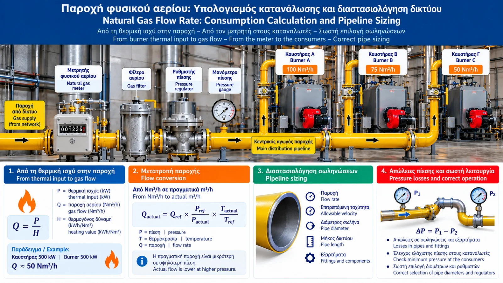
Natural Gas Flow Rate: Consumption Calculation and Pipeline Sizing

Correct sizing of a natural gas distribution network begins with a fundamental question: how much gas does the installation actually require at its design operating load?

In industrial boilers, steam generators, furnaces and combustion systems, insufficient flow capacity can cause pressure drops, limit available burner output or activate protective devices.

Conversely, excessive oversizing can increase installation costs without providing equivalent operational benefits.

Accurate engineering requires evaluation of fuel input, heating value, pressure, temperature, piping geometry and allowable pressure losses.

1. What Is Natural Gas Flow Rate?

Flow rate describes the quantity of gas passing through a point per unit time.

Common units include:

• m³/h: Volumetric flow at actual conditions.

• Nm³/h: Flow converted to defined normal reference conditions.

• Sm³/h: Flow converted to defined standard reference conditions.

• kg/h: Mass flow rate.

Reference conditions must be explicitly specified. Different suppliers and standards may use different reference temperatures.

2. Relationship Between Flow Rate and Thermal Input

Burner fuel input is related to gas flow and fuel heating value.

P = Q × H

where:

• P = fuel thermal input (kW).

• Q = reference volumetric flow (Nm³/h).

• H = heating value on the same reference basis (kWh/Nm³).

Therefore:

Q = P / H

The heating value basis must be consistent with the declared input rating.

Lower and higher heating values must not be mixed in the same calculation.

3. Example: 500 kW Industrial Burner

Assume:

• Fuel input = 500 kW.

• Illustrative lower heating value = 10 kWh/Nm³.

Then:

Q = 500 / 10 = 50 Nm³/h

The burner requires approximately 50 Nm³/h at the specified load under these assumptions.

The actual heating value depends on the gas composition and supply.

4. Example: 2,000 kW Industrial Boiler

An important distinction is whether the rated power refers to fuel input or useful heat output.

If 2,000 kW is the fuel input:

Q = 2,000 / 10 = 200 Nm³/h

If 2,000 kW is useful heat output and efficiency is assumed to be 90% on a consistent energy basis:

Fuel input = 2,000 / 0.90 = 2,222.2 kW

Therefore:

Q = 2,222.2 / 10 ≈ 222.2 Nm³/h

The difference demonstrates why the meaning of the rated capacity must be established before calculating fuel consumption.

5. Indicative Consumption Table

Assuming a lower heating value of 10 kWh/Nm³ and fuel input ratings:

These figures support preliminary estimates only. They are not pipe sizing values.

6. Calculating Total Installation Demand

For multiple gas consumers, design flow depends on their operating requirements.

Example:

• Burner A: 100 Nm³/h.

• Burner B: 75 Nm³/h.

• Burner C: 50 Nm³/h.

If all three can operate simultaneously at full load:

Qtotal = 100 + 75 + 50 = 225 Nm³/h

A different design demand may be justified where a documented operating interlock or other validated limitation prevents full simultaneous operation.

Diversity factors should not be applied arbitrarily.

7. Why Pressure Changes Actual Volumetric Flow

Natural gas is compressible.

For the same quantity of gas, actual volume changes with pressure and temperature.

Actual flow in m³/h may therefore differ substantially from reference flow in Nm³/h.

This distinction is essential when calculating gas velocity and pipe diameter.

8. Converting Nm³/h to Actual m³/h

With suitable compressibility correction:

Qactual = Qref × (P_ref / P_actual) × (T_actual / T_ref) × (Z_actual / Z_ref)

where:

• Qactual = flow at actual conditions.

• Qref = flow at reference conditions.

• P = absolute pressure.

• T = absolute temperature in kelvin.

• Z = gas compressibility factor.

For preliminary calculations near atmospheric pressure, an ideal gas approximation may be suitable where the required accuracy permits.

Example

Assume:

• Qref = 100 Nm³/h.

• Reference conditions = 0°C and 1.01325 bar absolute.

• Operating temperature = 20°C.

• Operating pressure = 2.01325 bar absolute.

• Zactual / Zref ≈ 1.

Then:

Qactual ≈ 100 × (1.01325 / 2.01325) × (293.15 / 273.15)

Qactual ≈ 54 m³/h

Actual volumetric flow is lower because of the higher operating pressure.

This is an approximate result based on the stated assumptions.

9. Flow, Cross-Sectional Area and Velocity

Mean gas velocity is related to actual volumetric flow and internal pipe area:

v = Qactual / A

where:

• v = mean velocity (m/s).

• Qactual = actual flow (m³/s).

• A = internal pipe area (m²).

For a circular pipe:

A = πD² / 4

D is the internal diameter in metres.

Reference flow in Nm³/h must not be inserted directly into this equation without conversion to actual operating conditions.

10. Gas Velocity Calculation Example

Assume:

Qactual = 100 m³/h

Convert to m³/s:

Qactual = 100 / 3,600 = 0.02778 m³/s

For an internal diameter of 100 mm:

D = 0.10 m

Pipe area:

A = π × 0.10² / 4 ≈ 0.00785 m²

Therefore:

v = 0.02778 / 0.00785 ≈ 3.54 m/s

This demonstrates the mathematical relationship. It does not establish that the diameter is suitable for a specific natural gas installation.

11. Why Velocity Alone Is Not Enough

Velocity is only one pipe sizing parameter.

Other factors include:

• Total pipe length.

• Internal diameter and material.

• Operating pressure.

• Available pressure difference.

• Gas density and properties.

• Fittings and local resistance.

• Minimum required pressure at consumers.

• Applicable codes and standards.

A pipe may have acceptable velocity but excessive pressure loss.

12. Understanding Pressure Drop

Gas flow through piping produces frictional and local resistance losses.

Pressure decreases along the flow direction.

Total pressure drop depends on pipe geometry, flow rate, gas properties and operating conditions.

Low-pressure systems may use approximate methods under defined assumptions. Networks with significant density variation require suitable compressible-flow calculations.

13. Losses Through Fittings and Equipment

Pressure losses arise not only in straight pipes but also in:

• Elbows.

• Tees and branches.

• Valves.

• Filters.

• Regulators.

• Meters.

• Safety equipment.

Losses may be evaluated using suitable local resistance coefficients or manufacturer data.

Control and safety equipment must be assessed using its actual specified performance.

14. Why Flow Capacity Becomes Insufficient at High Load

A system may operate normally at low demand but encounter problems at higher consumption.

Possible causes include:

• Undersized piping.

• Insufficient supply pressure.

• Excessive pressure losses.

• Contaminated filters.

• Unsuitable regulator.

• Restrictions in valves or meters.

• Simultaneous demand from multiple consumers.

Diagnosis should be based on actual measurements and the installation design.

15. Pipe Sizing in Branched Networks

In an industrial gas network, each section carries a different flow.

A main line may supply several consumers, while individual branches serve smaller loads.

Design flow must be determined for each section.

Example:

• Main line: 225 Nm³/h.

• Branch A: 100 Nm³/h.

• Branch B: 75 Nm³/h.

• Branch C: 50 Nm³/h.

Each branch diameter must be evaluated using its flow, operating pressure and allowable pressure loss.

16. Gas Flow and Modulating Burners

Many industrial burners modulate their firing rate according to thermal demand.

Their gas consumption therefore varies between specified minimum and maximum operating loads.

The network must supply the required maximum design flow, while meter and regulator selection must also account for lower operating flows.

17. Calculating Daily Gas Consumption

For constant flow:

V = Q × t

where:

• V = total gas volume.

• Q = flow rate.

• t = operating time.

Example:

A burner operates at an average flow of 80 Nm³/h for 10 hours.

V = 80 × 10 = 800 Nm³

Where flow varies, total consumption should be obtained by integrating flow over time or using an appropriate meter.

18. Converting Gas Volume to Energy

Energy content can be estimated from:

E = V × H

For example:

• V = 800 Nm³.

• H = 10 kWh/Nm³.

E = 8,000 kWh

This represents fuel energy on the selected heating-value basis, not necessarily the useful heat delivered by the installation.

19. Pre-Sizing Engineering Checklist

20. Standards and Engineering Requirements

Relevant references may include:

• EN 15001-1: Design, construction, inspection and testing of gas installations within its scope.

• EN 1775: Gas pipework for buildings within its scope.

• EN 676: Forced draught burners for gaseous fuels.

• EN 334: Gas pressure regulators.

• EN 12480, EN 12261 and EN 1359: Standards covering specific gas meter technologies.

National regulations, network operator requirements and manufacturer specifications must also be considered.

Conclusion

Natural gas flow calculation is the starting point for correct network sizing.

Fuel input and heating value provide an initial estimate of gas demand.

However, final pipe diameter selection cannot be based solely on Nm³/h or a general velocity rule.

It requires assessment of pressure, temperature, compressibility, pressure losses, fittings and simultaneous consumer operation.

Final sizing and any modifications to natural gas networks must be carried out by qualified engineering professionals in accordance with applicable technical and regulatory requirements.